Author: Nick Nickerson, Eosense
Gas analyzers have become increasingly more precise over the past 10 years with the adoption of laser-based sources and ultra-long path length optical cells. However, usually this has been at the cost of power consumption, making them difficult to easily deploy in the field, especially off-grid.
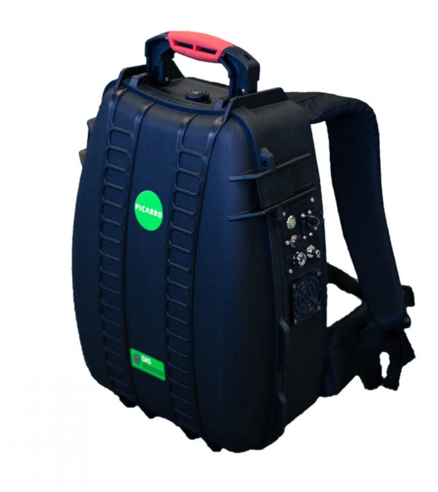
More recently, products like the new Picarro GasScouter have been designed to reduce the power consumption of these precision instruments and enhance their portability. For comparison, a standard Picarro analyzer usually draws about 200 W on average (for the analyzer and vacuum pump), whereas the GasScouter has an average draw of only 25 W. This low power consumption, plus excellent precision for CO2 and CH4 concentrations, make it an ideal instrument to measure greenhouse gas fluxes at off-grid field sites including agricultural fields and wetland sites.
Eosense's eosAC and eosMX-P automated soil flux chamber and multiplexer systems are being integrated with the Picarro GasScouter to offer a low power (9W average) solution for Picarro users to continuously monitoring of greenhouse gas fluxes. While the GasScouter does have an internal battery that allows it to run continuously for 8 hours, researchers may want to use the analyzer for longer-term, unattended deployments. We will show you how to power the GasScouter and eosAC system for off-grid unattended deployments, and how to build a solar power solution and enclosure using off the shelf parts you can usually find at your local hardware stores.
Power Requirements, Solar Panels and Batteries
The Picarro GasScouter and Eosense eosAC/eosMX-P system draws about 34 W of power on average. This means to run the two systems for a full day of operation we'll need about 816 Wh of energy (34 W * 25 h). We're going to have to size our solar panels based on this number and the peak sun for the location of our study. I've made these handy maps so you can see what the rough peak sun kWh/m2/d values are for your location during the winter and summer solstices.

Global peak solar for June (Summer Solstice) accounting for average weather conditions. Data from NASA SSE Release 6.0 (July 1983 – June 2005).

Global peak solar for December (Winter Solstice) accounting for average weather conditions. Data from NASA SSE Release 6.0 (July 1983 – June 2005).
Since we're going to be doing our testing in Nova Scotia, I am going to do a few quick calculations based on the summer (4-6 kWh/m2/d) and winter (2-4 kWh/m2/d) solstices (see maps above).
Summer = 816 Wh/4-6 kWh/m2/d = 136-204 W
Winter = 816 Wh/2-4 kWh/m2/d = 204-408 W
So if we only really want to deploy our system in the summer we can likely get away with 200 W of solar power, and if we want to extend our deployment into the winter then we should probably double our solar panels power output to 400 W.
Obviously we'll need to store this solar energy (unless we're hanging out in the Arctic during the summer solstice). The Picarro GasScouter has a 223 Wh Li-Ion battery that will give us about six and a half hours (6.5 h) of backup, but not enough to make it through the night. So we're going to supplement that with a few marine deep cycle batteries, but how many? To be safe we're going to say we want the system to run for 3 days of absolutely miserable weather (no solar charge), which will be about 2450 Wh of energy at 12 V. Remembering back to your first year physics, P=IV, so we need about 200 Amp Hours of battery. But safety first, if we drain a lead acid battery it's not going to charge back up, so we're going to add 50% to that and assume we need 300 Ah to keep the system safe and sound. Checking out our local suppliers, it looks like we can get three 115 Ah deepcycle batteries for about $450 CAD, not bad for just over 3 days of total autonomy.
Building the Enclosure
The easiest thing for most people to get a hold of will be a rubber/plastic garden tool shed, which can be found at most local hardware stores. The critical consideration is to make sure it has inside dimensions of at least 51 cm depth by 115 cm width by 60 cm height (approx. 20"x45"x24"); this should allow enough space for your batteries, Picarro GasScouter and eosMX-P multiplexer to fit comfortably inside.

We bought a plastic tool shed from the local hardware store, assembled it and used a hole saw to make two holes in the side of the shed to allow the eosAC tubing and cables to pass from the shed out to their field location. Since the edges of the shed are sharp after cutting, two small sections of PVC pipe were glued (without elegance) into the holes using outdoor caulking.
This was really all that was required for us to ready the enclosure for field use. When making your enclosure you'll obviously need to consider the local weather and other environmental factors of the field site, so you may need to add extra caulking, weather stripping or other similar hardware in order to make the enclosure tight enough to keep your equipment safe.
Wiring the Enclosure for Solar & Batteries
We used a ProStar-30 solar charge controller in our enclosure to ensure that the solar panels are charging the batteries properly. The two large (15 gauge wire) cables on the left will go to the solar panels, the yellow cable (also 15 gauge wire) will connect to the batteries and lastly the two grey cables with connectors are meant to go to the GasScouter and eosMX-P.
 When connecting the various components (batteries, solar and equipment) to the charge controller the recommended order is.
- Connect batteries
- Connect solar
- Connect load (equipment)
In order to make a good connection on the batteries, a few battery terminal clamps were bought. These clamps are appropriately sized for the battery terminals, and also have a user adjustable clamp on the back where we can insert and clamp down on the wires from the charge controller. Eosense's Electrical Engineering Manager Darren Wall points out that when using multiple batteries they ideally should be attached with a special configuration to equalize the wear (charging/discharging) on each individual battery. Shown below is an example illustration of the connection for 3 batteries.
Next we connected the solar panels to the charge controller. Since our panels were in full sun during deployment we connected both positive leads to the solar panels first, and then the two negative leads. If we had connected the solar panels one at a time we would have had one live cable after connecting the first one — making for a dangerous situation when connecting panel number two.

Finally we plugged the two custom cables into the GasScouter and eosMX-P and powered on the system! Everything looks like it's humming along smoothly.

We deployed the GasScouter and eosAC system at Dalhousie University's BioEnvironmental Engineering Centre (BEEC). BEEC is a research and demonstration site operated jointly by the Faculty of Agriculture's Engineering Department and Dalhousie University's Department of Biological Engineering.
We set up the system on a constructed wetland at the BEEC site (normally used for studying filtering of biosolids) with the purpose of monitoring the CO2 and methane emissions from the wetland in comparison with the emissions from the raised land near the wetland (where the shed and equipment was set up — which we'll call the upland from now on).

Our shed, solar panels and batteries were set up on the upland portion of the site. We installed four eosAC chambers at the site, three in the wetland soil (approximately 30-40 cm from each other) and one on the upland, as seen below. Each chamber had a 10 cm tall soil collar, inserted approximately 7 cm into the soil (3 cm exposed lip) and 15 meters of tubing from the chamber to the shed containing the GasScouter and eosMX chamber multiplexer.

Using the eosLink-MX software, the chambers were set to each do 10 minute long measurements in sequence (1,2,3,4) with a 60 second purge time before chamber closure.
Performance and Preliminary Flux Data
We visited the field site approximately 5 days after the initial deployment and found the system was 50% working (just the eosMX-P in this case). After some troubleshooting of the system we had found that the GasScouter suffered from a blown fuse in its internal battery; probably because of a low voltage in the deep-cycle batteries after a few days of cloud, causing a large increase in required charge current. In order to prevent this in future, Darren did a quick calculation and determined that we should put a fastblow 7 Amp fuse in line with the GasScouter power. This way, if the GasScouter tries to draw too much current, the 7 Amp fuse blows rather than the fuse in the Lithium Ion battery pack (not user replaceable).
After repairing the fuse in our electronics shop, we took the system back to the field for the weekend to gather a bit more data before it had to be pulled for other uses.
During the course of the experiment, we observed a temperature correlated CO2 flux in all of the plots; although the upland chamber (Chamber 1) demonstrated a weaker temperature response likely due to very dry soil.

Fluxes of carbon dioxide and chamber temperature during the deployment period. Note the strong positive correlation between temperature and CO2 flux.

Chamber temperature versus flux for the wetland (blue) and upland (green) showing the upland had a reduced temperature response because of dry conditions.
There was consistent methane uptake from the upland chamber, whereas the wetland chambers showed consistent methane emission with an average rate of 19.85 nmol/m2/s and a standard deviation of 54.7 nmol/m2/s with a positively skewed distribution.

Chamber methane fluxes for the wetland (blue, red, green) and upland (black) sites. Note that the wetland is plotted on the left y-axis and is always emitting whereas the upland is plotted on the right y-axis and has a consistent uptake.
During our second deployment we had a small rainfall event that drove massive increases in methane flux for the wetland chambers (see above), but with almost no change in the methane dynamics for the upland chamber. It's unclear if this was an event that caused a short-term increase in the production of methane, or simply drove methane out of the wetland soil pores by volume replacement. Some of the flux curves suggest ebullition of methane, which is more consistent with the volume replacement theory.

eosAnalyze-AC screenshots showing a well behaved increase in CO2 concentration (left) and a CH4 time series that is consistent with ebullition (right).
That's all for the data for now. We'll be presenting the fully worked up data at the ASA, CSSA & SSSA International Annual Meeting in Phoenix from November 6-9. The poster will be in the "General Wetland Soils Poster 1" session from 14:30-16:30 on Wednesday, November 9th.
Conclusion
Our enclosure and solar panel system were able to keep the system dry and powered, although an increase in the safety factor on both the batteries and solar supply is recommended as it's not guaranteed that the solar for your site will be consistent with the mean values we presented.
Luckily we experienced the low-voltage fuse issue ourselves, and now can recommend that users install and additional fuse (fast-blow, 7 Amps) before the GasScouter to protect its internal fuses and electrical components.
The data shows expected trends, including a positive correlation between CO2 flux, temperature and methane release in the wetland. Interestingly we observed very high rates of methane release after a single rain event, which could be caused by release of methane from the soil pore space during percolation of rainwater.
Acknowledgements
Thanks to David Burton and Peter Harvard for hosting us at the BEEC site during this study; and to David Kim-Hak and the technical team at Picarro for their technical assistance during the deployment.
| Attachment | Size |
|---|---|
| NASA-SSE-1.jpg (67.25 KB) | 67.25 KB |
| NASA-SSE-2.jpg (70.81 KB) | 70.81 KB |
| Enclosure.jpg (43.28 KB) | 43.28 KB |
| connectors.jpg (40.61 KB) | 40.61 KB |
| chargecontroller.jpg (22.41 KB) | 22.41 KB |
| solarpanels.jpg (55.66 KB) | 55.66 KB |
| shed.jpg (50.4 KB) | 50.4 KB |
| shed-2.jpg (129.34 KB) | 129.34 KB |
| flux-data.jpg (54.85 KB) | 54.85 KB |
| flux-data2.jpg (51.29 KB) | 51.29 KB |
| MethaneEmissions.jpg (48.3 KB) | 48.3 KB |
| measurements.jpg (53.53 KB) | 53.53 KB |